2 Data

2.1 Technical Description

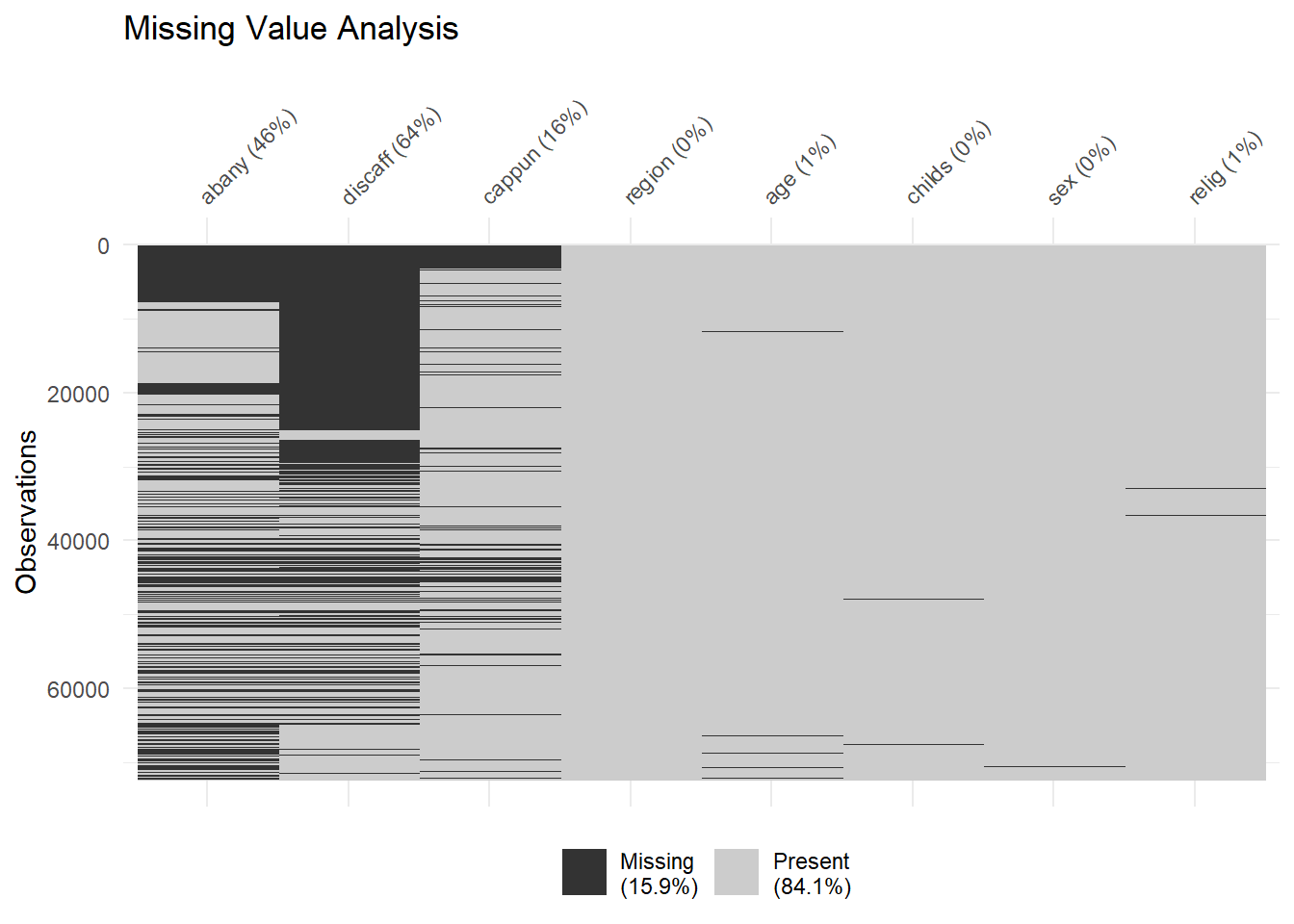
The data will be retrieved from the General Social Survey (GSS), a nationally representative survey of US adults run by the National Opinion Research Center at the University of Chicago, with surveys that ran every one to two years dating back to 1972 on a wide range of topics, with at least 1,500 respondents in every sample. The data can be downloaded with the use of their API and the packages gssr and gssrdoc, and contains demographic information on respondents. The major flaw in this data source is that it is almost entirely self-reported survey data. Although this is inevitable when working with survey and social data, it is particularly notable that almost all of the GSS data is the result of self-reported. Furthermore, while at the start the survey ran every year, after 1994, the GSS switched to running on every even-numbered year. This presented significant problems during the COVID pandemic beginning in 2020. Any time series analysis will have to take into account these uneven time points.

2.1.1 Data Sources

About the GSS
In-browser data explorer for the GSS
The data is accessed through the gssr package

2.2 Data Cleaning on Key Variables

We select the following demographic variables for our analysis:

sex
age
race
relig: current religious preference
polviews: political/social views (think of self as liberal or conservative)
reg16: region of residence at age 16
reg: region of interview
wrkstat: current employment status

We select specific abortion, affirmative action, and capital punishment variables. With regards to abortion, we choose seven abortion variables each representing a different reason a woman could be seeking an abortion and respondents’ opinion (Yes, No, NA) on whether a woman should be able to obtain a legal abortion for such a reason.

For affirmative action, we look at two opinion survey variables, discaff (which asks whether the respondent believes that white people are harmed by affirmative action), and affrmact (which asks about the respondents general support for affirmative action in the workplace).

For capital punishment, we look at cappun, which asks the respondents opinion on whether the death penalty should be a punishment for a murder conviction.

We clean and transform the data by mutating categorical variables into factors with meaningful labels. We also remove the rows with NA values in the abortion-related columns. This is because we discovered through data exploration that the NA values pertaining to these variables represent inapplicable responses. Therefore, we remove these rows to ensure that we only use relevant and complete data for further analysis. Similarly, inapplicable responses for capital punishment and affirmative action questions were discarded, as well as NA values for the demographic indicators we are investigating.

2.3 Missing value analysis

2.3.1 Overall

Code

library(gssr)
library(gssrdoc)
library(naniar)
library(dplyr)
library(ggplot2)
library(forcats)
data(gss_all)
gss_all |>
  select(abany, discaff, cappun, region, age, childs, sex, relig) |>
  vis_miss() + 
  ggtitle("Missing Value Analysis")

Above, we can see a quick visualization of the primary variables - both dependent and independent - and which ones are missing. Not all questions were asked in all years of the survey. The main pattern here is that our response variables (abany = “Whether it should be possible for a pregnant woman to obtain a legal abortion if the woman wants it for any reason”; discaff = “What do you think the chances are these days that a white person won’t get a job or promotion while an equally or less qualified black person gets one instead?”; cappun = “Do you favor or oppose the death penalty for persons convicted of murder?”) are much more likely to be missing. This is because not every question was asked every year of the survey, and respondents are more likely to refuse to answer controversial questions than demographic data such as region, age, etc.

2.3.2 Abortion: Missing Variables

In our analysis of public opinion on abortion using the GSS data, we initially noticed a significant increase in the proportion of missing (NA) responses on abortion-related variables in some years, which led to suspicious decreases in the percentage of respondents in favor of abortion. Upon further investigation, we found that the missing responses were predominantly categorized as “NA(i)” (inapplicable), with only a small percentage of “NA(d)” (don’t know) responses, which would be expected in a survey of this nature. This is the result of the survey-ballot method behind the GSS, where not all questions are asked to all survey participants. Additionally, we decided to remove the other NA values at this time, as the other responses made up a very small proportion of answers. This decision was crucial, as including these NAs distorted the true proportions of “yes” and “no” responses, leading to potentially misleading conclusions about trends in abortion attitudes over time.

Below is a graph showing the percentage of missing values in each of the abortion-related variables we investigate in our analysis. Note that all the variables have a high percentage of missing values around 45% for “abortion for any reason” and around 35% for all other variables, as not all variables were included on all slates. Additionally, note that most of the missing values are inapplicable responses with over 90% of all missing values being inapplicable responses.

Code

gss_ab = gss_all |>
  select(c(year, abdefect, abnomore, abhlth, abpoor, abrape, absingle, abany, sex, age, race, degree, relig, relig16, marital, partyid, polviews, childs, region, reg16))

abdefect = data.frame(base::table(haven::as_factor(gss_ab$abdefect, levels = "labels"))) |> mutate(nrow = sum(Freq)) |> mutate(Perc = round(Freq*100/nrow,2), abdefect = Var1) |> select(abdefect, Freq, nrow, Perc)|> filter(!(abdefect %in% c("yes","no") | Freq ==0)) |> select(abdefect, Perc) |> mutate(response = abdefect, reason = rep("abdefect", 4)) |> select(reason,response, Perc)


abrape = data.frame(base::table(haven::as_factor(gss_ab$abrape, levels = "labels"))) |> mutate(nrow = sum(Freq)) |> mutate(Perc = round(Freq*100/nrow,2), abrape = Var1) |> select(abrape, Freq, nrow, Perc)|> filter(!(abrape %in% c("yes","no") | Freq ==0)) |> select(abrape, Perc) |> mutate(response = abrape, reason = rep("abrape", 4)) |> select(reason,response, Perc)

abhlth = data.frame(base::table(haven::as_factor(gss_ab$abhlth, levels = "labels"))) |> mutate(nrow = sum(Freq)) |> mutate(Perc = round(Freq*100/nrow,2), abhlth = Var1) |> select(abhlth, Freq, nrow, Perc)|> filter(!(abhlth %in% c("yes","no") | Freq ==0)) |> select(abhlth, Perc) |> mutate(response = abhlth, reason = rep("abhlth", 4)) |> select(reason,response, Perc)

abpoor = data.frame(base::table(haven::as_factor(gss_ab$abpoor, levels = "labels"))) |> mutate(nrow = sum(Freq)) |> mutate(Perc = round(Freq*100/nrow,2), abpoor = Var1) |> select(abpoor, Freq, nrow, Perc)|> filter(!(abpoor %in% c("yes","no") | Freq ==0)) |> select(abpoor, Perc) |> mutate(response = abpoor, reason = rep("abpoor", 4)) |> select(reason,response, Perc)

abnomore = data.frame(base::table(haven::as_factor(gss_ab$abnomore, levels = "labels"))) |> mutate(nrow = sum(Freq)) |> mutate(Perc = round(Freq*100/nrow,2), abnomore = Var1) |> select(abnomore, Freq, nrow, Perc)|> filter(!(abnomore %in% c("yes","no") | Freq ==0)) |> select(abnomore, Perc) |> mutate(response = abnomore, reason = rep("abnomore", 4)) |> select(reason,response, Perc)

absingle = data.frame(base::table(haven::as_factor(gss_ab$absingle, levels = "labels"))) |> mutate(nrow = sum(Freq)) |> mutate(Perc = round(Freq*100/nrow,2), absingle = Var1) |> select(absingle, Freq, nrow, Perc)|> filter(!(absingle %in% c("yes","no") | Freq ==0)) |> select(absingle, Perc) |> mutate(response = absingle, reason = rep("absingle", 4)) |> select(reason,response, Perc)

abany = data.frame(base::table(haven::as_factor(gss_ab$abany, levels = "labels"))) |> mutate(nrow = sum(Freq)) |> mutate(Perc = round(Freq*100/nrow,2), abany = Var1) |> select(abany, Freq, nrow, Perc)|> filter(!(abany %in% c("yes","no") | Freq ==0)) |> select(abany, Perc) |> mutate(response = abany, reason = rep("abany", 4)) |> select(reason,response, Perc)

NA_percentage = rbind(abhlth, abrape, abdefect, abpoor, abnomore, absingle, abany)

NA_percentage_b = NA_percentage |> 
  mutate(response = factor(response, levels = c("iap", "don't know", "no answer", "skipped on web"))) |> 
  mutate(reason = case_when(reason == "abhlth" ~ "mother's health",
                                                 reason == "abrape" ~ "rape",
                                                 reason == "abdefect" ~ "birth defect",
                                                 reason == "abpoor" ~ "financial hardship",
                                                 reason == "abnomore" ~ "married-no more children",
                                                 reason == "absingle" ~ "not married",
                                                 reason == "abany" ~ "any reason")) |>
  mutate(response = recode(response, iap = "inapplicable"))


inv = NA_percentage_b |> group_by(reason) |> summarize(sum(Perc)) |> arrange(desc(`sum(Perc)`)) |> select(reason)

                          
ggplot(NA_percentage_b |> mutate(reason = factor(reason, levels = inv$reason)), aes(x=reason, y= Perc, fill = response)) +
  geom_col() +
  labs(x = "Reason for abortion", y = "Percentage of Missing Values (NA) in the Responses", title = "Percentage of Missing Values (NA) in Responses to Abortion Questions by NA Label", fill = "Response") +
  theme_bw(12) +
  theme(plot.title = element_text( size = 20))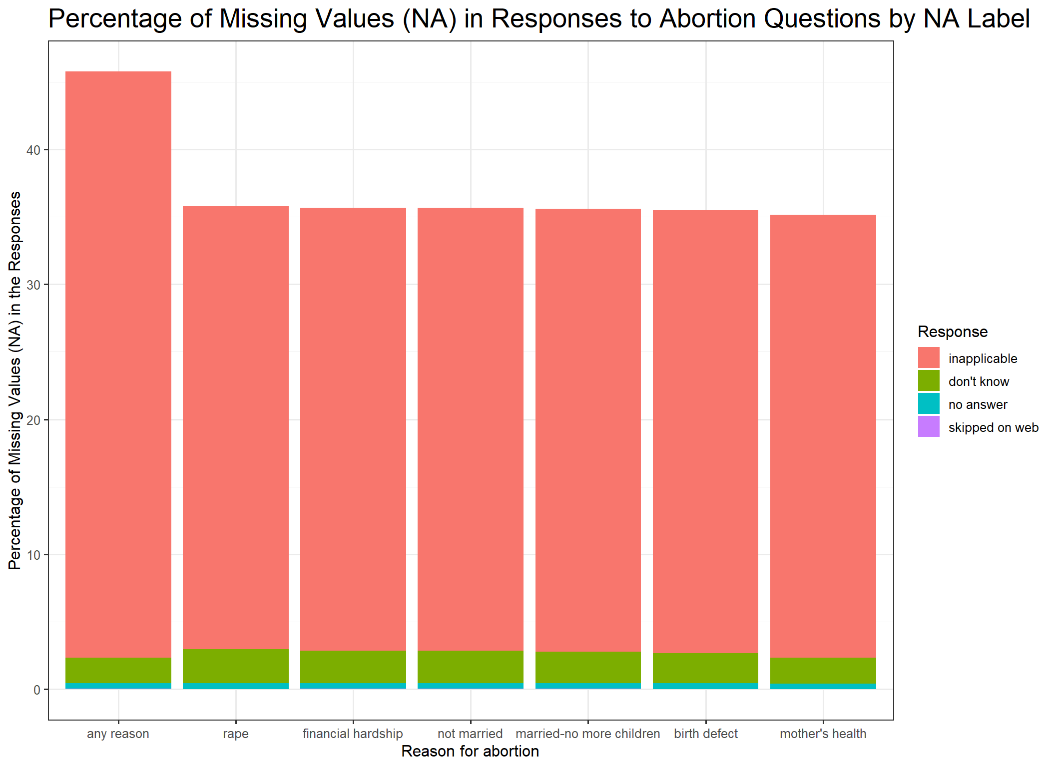

2.3.3 Affirmative Action: Missing Values

Code

gss_ad <- gss_all |> 
  select(discaff, affrmact)

ggplot(gss_ad, aes(y = fct_rev(fct_infreq(haven::as_factor(discaff)))))+
  geom_bar() + 
  ggtitle("Value Breakdown of 'discaff' Variable") +
  labs(y = "Possible Responses to 'discaff'", x = "Count") +
  theme_bw()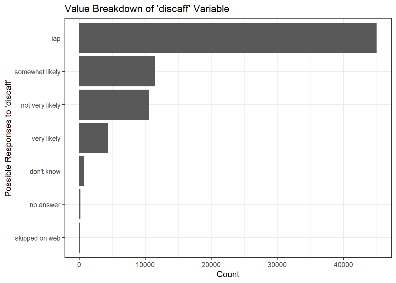

Code

ggplot(gss_ad, aes(y = fct_rev(fct_infreq(haven::as_factor(affrmact))))) + 
  geom_bar() + 
  ggtitle("Value Breakdown of 'affrmact' Variable") +
  labs(y = "Possible Responses to 'affrmact'", x = "Count") +
  theme_bw()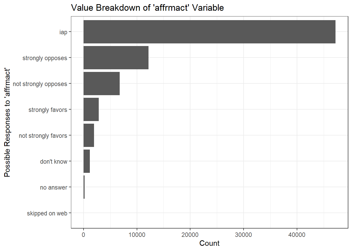

Similar to the abortion questions, as there are several possible slates of questions asked to respondents, not all survey participants are asked all questions. We will therefore discard the inapplicable answers (iap), as they did not participate in these questions; and the “don’t know” values make up a small enough proportion of responses to be irrelevant to analyses.

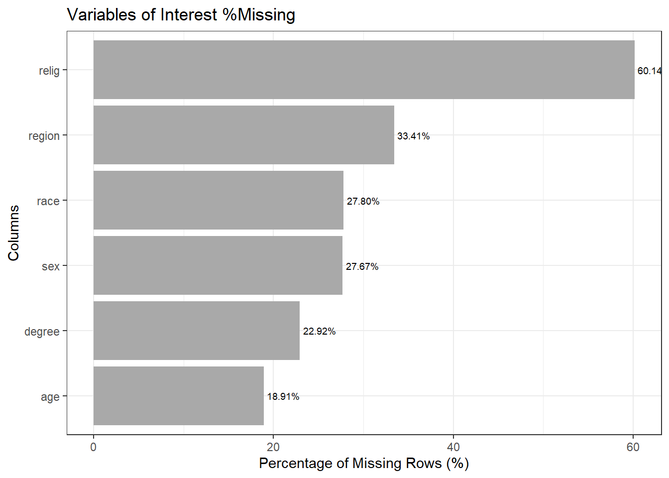
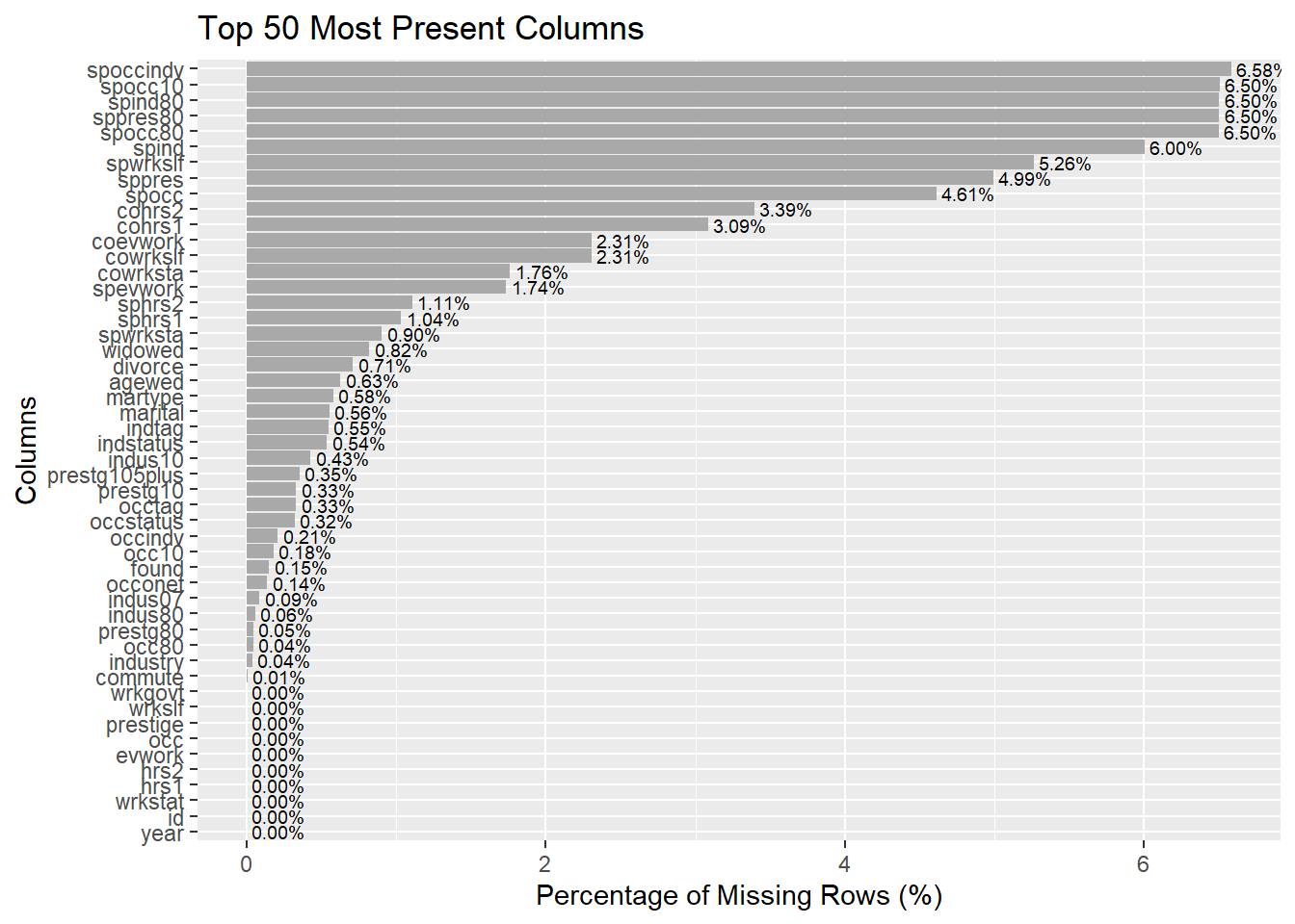
2.3.4 Capital Punishment (cappun) missing row analysis

The missing data analysis reveals that there are significant gaps in the information collected for this survey. The variable with the highest rate of missing values is religion, with 60.14% of responses lacking this data point. Region also has a high rate of missingness at 33.41%. Other variables with substantial missing information include degree (22.92% missing), sex (27.67% missing), and race (27.80% missing). The variable with the lowest rate of missing data is age, but even here 18.91% of responses are incomplete. These high levels of missingness across multiple key demographic variables could introduce bias and limit the conclusions that can be drawn from the analysis. It will be important to carefully consider how to address these gaps, whether through imputation techniques or by restricting the analysis to only complete cases, in order to obtain reliable insights from the Capital Punishment dataset.

Code

cp <- gss_all |> filter(cappun==1 | cappun==2)

cp_df <- data.frame(
  column = names(colSums(is.na(cp))),
  missing_count = sort(colSums(is.na(cp))),
  total_responses = nrow(cp)
)

# variables of interest
cp_df_2 <- cp_df |> filter(column %in% c('age', 'race', 'sex', 'region', 'relig', 'degree'))

# percentage of missing data
cp_df$missing_percentage <- (cp_df$missing_count / cp_df$total_responses) * 100
cp_df_2$missing_percentage <- (cp_df_2$missing_count / cp_df_2$total_responses) * 100

cp_df_sorted <- cp_df |> arrange(missing_percentage)

cp_df_2_sorted <- cp_df_2 |> 
  arrange(missing_percentage) |> 
  mutate(column = factor(column, levels = column))

top_50_present <- cp_df_sorted |> 
  slice_head(n = 50) |> 
  mutate(column = factor(column, levels = column))

ggplot(top_50_present, aes(x = column, y = missing_percentage)) +
  geom_bar(stat = "identity", fill = "darkgrey") +
  coord_flip() +
  labs(
    title = 'Top 50 Most Present Columns',
    x = "Columns",
    y = "Percentage of Missing Rows (%)"
  ) +
  geom_text(
    aes(label = sprintf("%.2f%%", missing_percentage)), 
    position = position_dodge(width = 0.9),
    hjust = -0.1,
    size = 2.5
  )

Code

ggplot(cp_df_2_sorted, aes(x = column, y = missing_percentage)) +
  geom_bar(stat = "identity", fill = "darkgrey") +
  coord_flip() +
  labs(
    title = 'Variables of Interest %Missing',
    x = "Columns",
    y = "Percentage of Missing Rows (%)"
  ) +
  geom_text(
    aes(label = sprintf("%.2f%%", missing_percentage)), 
    position = position_dodge(width = 0.9),
    hjust = -0.1,
    size = 2.5
  ) + theme_bw()