3 Results

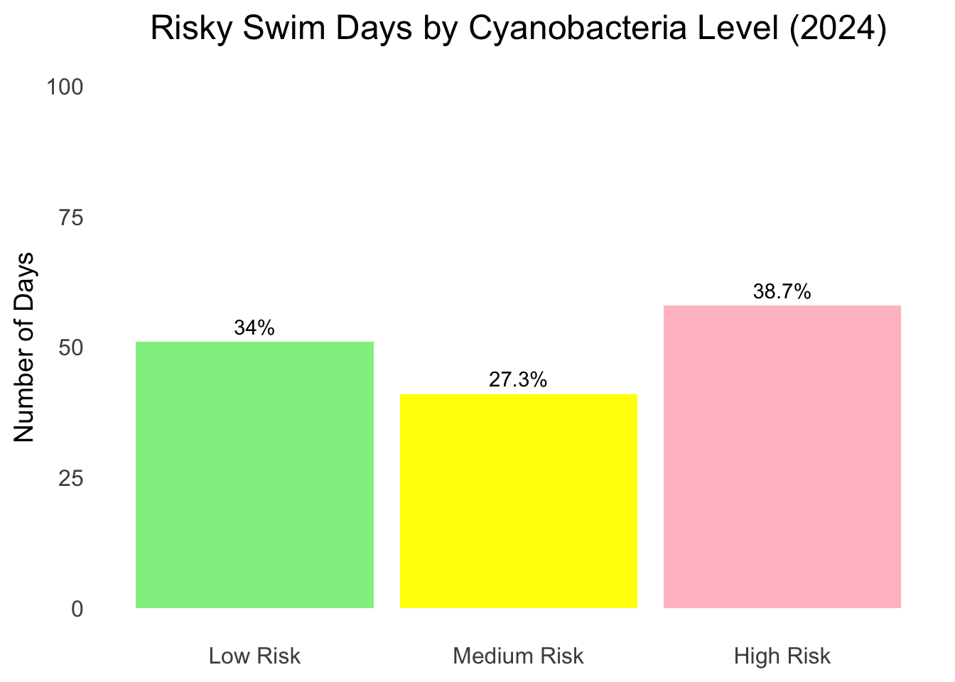
3.1 How many days of the 2024 season are cyanobacteria levels safe for swimming in the Charles River?

The World Health Organization (WHO) defines <20,000 cyanobacteria cells/mL as low risk. The Massachusetts Advisory Level for high risk is >70,000 cyanobacteria cells/mL. Medium risk is between 20,000 and 70,000.

In 2024, cyanobacteria levels were low risk on 51 days (34%), medium risk on 41 days (27%), and high risk on 58 days (39%).

Code

library(dplyr)
library(ggplot2)
library(tidyr)
library(lubridate)

# 2024
water2024<-read.csv('./data/crbuoy2024.csv')
water2024_summary <- water2024 |> 
  select(date, temp.c, `do..mg.l.`, `est.chl.a..ug.l.`, `est..cyano..cells.ml.`) |> 
  group_by(date) |> 
  summarize(
    avg_temp = pmax(mean((temp.c * 9/5) + 32, na.rm = TRUE),0),
    avg_oxygen = pmax(mean(`do..mg.l.`, na.rm = TRUE),0),
    avg_chloro = pmax(mean(`est.chl.a..ug.l.`, na.rm = TRUE),0),
    avg_est_cyano = pmax(mean(`est..cyano..cells.ml.`, na.rm = TRUE),0)
  )
water2024_summary$date <- as.Date(water2024_summary$date, format = "%m/%d/%Y")

water2024_summary <- water2024_summary |>
  mutate(
    hab_risk = case_when(
      avg_est_cyano < 20000 ~ "Low Risk",
      avg_est_cyano >= 20000 & avg_est_cyano < 70000 ~ "Medium Risk",
      avg_est_cyano >= 70000 ~ "High Risk"                       
    ),
    hab_risk = factor(hab_risk, levels = c("Low Risk", "Medium Risk", "High Risk"))
  )

# Count the number of days for each risk category
risk_counts2024 <- water2024_summary |>
  count(hab_risk)

total_count2024 <- sum(risk_counts2024$n)
risk_counts2024 <- risk_counts2024 |>
  mutate(
    percentage = (n / total_count2024) * 100  # Calculate percentage for each category
  )

ggplot(risk_counts2024, aes(x = hab_risk, y = n, fill = hab_risk)) +
  geom_bar(stat = "identity", show.legend = FALSE) +
  geom_text(aes(label = paste0(round(percentage, 1), "%")), vjust = -0.5) +  # Add percentage labels
  scale_fill_manual(values = c("Low Risk" = "lightgreen", "Medium Risk" = "yellow", "High Risk" = "pink", "Unknown" = "gray")) +
  scale_y_continuous(limits = c(0, 100)) +
  labs(
    title = "Risky Swim Days by Cyanobacteria Level (2024)",
    x = "Risk Category",
    y = "Number of Days"
  ) +
  labs(x = NULL) +
  theme_minimal(base_size = 15) +
    theme(
        plot.title = element_text(size = 18, hjust = 0.5),  # Title style
        axis.title = element_text(size = 14),  # Axis titles
        axis.text = element_text(size = 12),  # Axis labels
        panel.grid.major = element_blank(),  # Remove major grid lines
        panel.grid.minor = element_blank(),  # Remove minor grid lines
      )

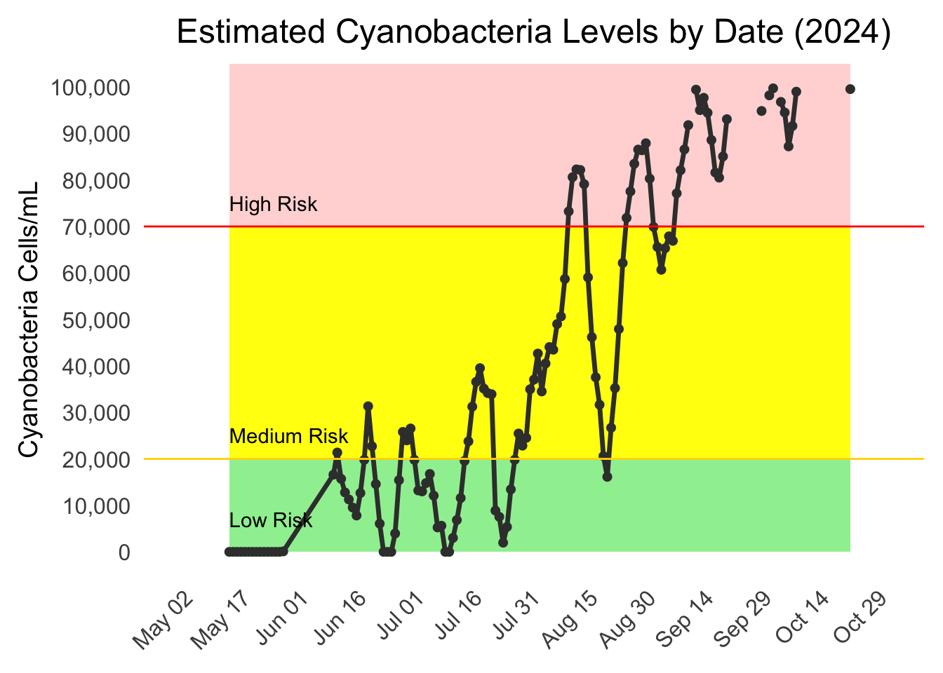
3.1.1 Estimated Cyanobacteria Levels in 2024

Cyanobacteria levels increased over the course of the summer, with several noteworthy blooms towards the end of the season.

Code

ggplot(water2024_summary, aes(x = date, y = avg_est_cyano)) +
  geom_rect(aes(xmin = min(date), xmax = max(date),
                ymin = 0, ymax = 20000),
            fill = "lightgreen", alpha = 0.03) +
  geom_rect(aes(xmin = min(date), xmax = max(date),
                ymin = 20000, ymax = 70000),
            fill = "yellow", alpha = 0.03) +
  geom_rect(aes(xmin = min(date), xmax = max(date),
                ymin = 70000, ymax = Inf),
            fill = "pink", alpha = 0.03) +
  geom_line(color = "#3b3b3b", size = 1.2) +
  geom_point(color = "#3b3b3b", size = 1.8) + 
  geom_hline(yintercept = 20000, linetype = "solid", color = "gold") +
  geom_hline(yintercept = 70000, linetype = "solid", color = "red") +
  annotate("text", x = min(water2024_summary$date), y = 7000,
           label = "Low Risk", hjust = 0) +
  annotate("text", x = min(water2024_summary$date), y = 25000,
           label = "Medium Risk", hjust = 0) +
  annotate("text", x = min(water2024_summary$date), y = 75000,
           label = "High Risk", hjust = 0) +
  scale_y_continuous(
    limits = c(0,100000),
    labels = scales::comma,
    breaks = seq(0, max(water2024_summary$avg_est_cyano), by = 10000)
    ) +
    scale_x_date(
    limits = as.Date(c("2024-05-01", "2024-11-01")),
    date_labels = "%b %d", 
    date_breaks = "15 day") +
  labs(title = "Estimated Cyanobacteria Levels by Date (2024)",
       x = NULL,
       y = "Cyanobacteria Cells/mL") +
  theme_minimal(base_size = 15) +
  theme (
    plot.title = element_text(size = 18, hjust = 0.5),  # Title style
    axis.title = element_text(size = 14),  # Axis titles size
    axis.text = element_text(size = 12),  # Axis labels size
    axis.text.x = element_text(angle = 45, hjust = 1),  # Rotate X-axis labels for clarity
    panel.grid.major = element_blank(),  # Remove major grid lines
    panel.grid.minor = element_blank(),  # Remove minor grid lines
    plot.margin = margin(10, 10, 10, 10)  # Adjust margins for better spacing
  )

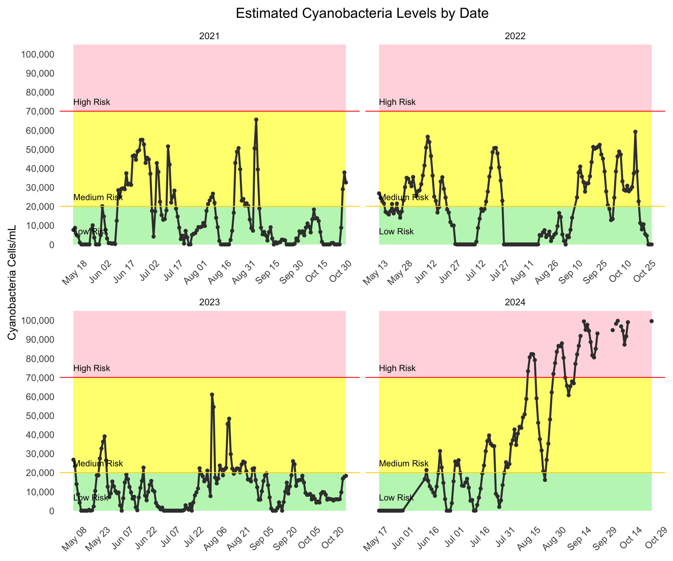
3.2 Historical Analysis (2021-2024)

In 2021, 2022, and 2023, there were zero high risk days. Additionally, the percentage of low risk days was much higher than 2024 with 71%, 54%, and 82% low risk days in the season, respectively. This suggests that overall safe-for-swim days in the Charles River may be closer to 60%, and that 2024 was an outlier year with late season cyanobacteria blooms.

Code

# 2021
water2021<-read.csv('./data/crbuoy2021.csv')
water2021_summary <- water2021 |> 
  select(date, temp.c, `do..mg.l.`, `est.chl.a..ug.l.`, `est..cyano..cells.ml.`) |> 
  group_by(date) |> 
  summarize(
    avg_temp = pmax(mean((temp.c * 9/5) + 32, na.rm = TRUE),0),
    avg_oxygen = pmax(mean(`do..mg.l.`, na.rm = TRUE),0),
    avg_chloro = pmax(mean(`est.chl.a..ug.l.`, na.rm = TRUE),0),
    avg_est_cyano = pmax(mean(`est..cyano..cells.ml.`, na.rm = TRUE),0)
  )
water2021_summary$date <- as.Date(water2021_summary$date, format = "%m/%d/%Y")

# 2022
water2022<-read.csv('./data/crbuoy2022.csv')
water2022_summary <- water2022 |> 
  select(date, temp.c, `do..mg.l.`, `est.chl.a..ug.l.`, `est..cyano..cells.ml.`) |> 
  group_by(date) |> 
  summarize(
    avg_temp = pmax(mean((temp.c * 9/5) + 32, na.rm = TRUE),0),
    avg_oxygen = pmax(mean(`do..mg.l.`, na.rm = TRUE),0),
    avg_chloro = pmax(mean(`est.chl.a..ug.l.`, na.rm = TRUE),0),
    avg_est_cyano = pmax(mean(`est..cyano..cells.ml.`, na.rm = TRUE),0)
  )
water2022_summary$date <- as.Date(water2022_summary$date, format = "%m/%d/%Y")

# 2023
water2023<-read.csv('./data/crbuoy2023.csv')
water2023_summary <- water2023 |> 
  select(date, temp.c, `do..mg.l.`, `est.chl.a..ug.l.`, `est..cyano..cells.ml.`) |> 
  group_by(date) |> 
  summarize(
    avg_temp = pmax(mean((temp.c * 9/5) + 32, na.rm = TRUE),0),
    avg_oxygen = pmax(mean(`do..mg.l.`, na.rm = TRUE),0),
    avg_chloro = pmax(mean(`est.chl.a..ug.l.`, na.rm = TRUE),0),
    avg_est_cyano = pmax(mean(`est..cyano..cells.ml.`, na.rm = TRUE),0)
  )
water2023_summary$date <- as.Date(water2023_summary$date, format = "%m/%d/%Y")

# 2024
water2024<-read.csv('./data/crbuoy2024.csv')
water2024_summary <- water2024 |> 
  select(date, temp.c, `do..mg.l.`, `est.chl.a..ug.l.`, `est..cyano..cells.ml.`) |> 
  group_by(date) |> 
  summarize(
    avg_temp = pmax(mean((temp.c * 9/5) + 32, na.rm = TRUE),0),
    avg_oxygen = pmax(mean(`do..mg.l.`, na.rm = TRUE),0),
    avg_chloro = pmax(mean(`est.chl.a..ug.l.`, na.rm = TRUE),0),
    avg_est_cyano = pmax(mean(`est..cyano..cells.ml.`, na.rm = TRUE),0)
  )
water2024_summary$date <- as.Date(water2024_summary$date, format = "%m/%d/%Y")

# Drop hab_risk column to combine years
water2024_summary <- water2024_summary[, !(names(water2024_summary) %in% "hab_risk")]

# Combine the data
water_data <- rbind(
  transform(water2021_summary, year = 2021),
  transform(water2022_summary, year = 2022),
  transform(water2023_summary, year = 2023),
  transform(water2024_summary, year = 2024)
)

decor_data <- water_data |>
  group_by(year) |>
  summarize(
    xmin = min(date),
    xmax = max(date),
    low_risk_label_x = min(date),
    medium_risk_label_x = min(date),
    high_risk_label_x = min(date),
    low_risk_label_y = 7000,
    medium_risk_label_y = 25000,
    high_risk_label_y = 75000
  )

# Create the 2x2 grid of plots using facet_wrap
ggplot(water_data, aes(x = date, y = avg_est_cyano)) +
  geom_rect(
    data = decor_data,
    aes(xmin = xmin, xmax = xmax, ymin = 0, ymax = 20000),
    fill = "lightgreen",
    alpha = 0.6,
    inherit.aes = FALSE
  ) +
  geom_rect(
    data = decor_data,
    aes(xmin = xmin, xmax = xmax, ymin = 20000, ymax = 70000),
    fill = "yellow",
    alpha = 0.6,
    inherit.aes = FALSE
  ) +
  geom_rect(
    data = decor_data,
    aes(xmin = xmin, xmax = xmax, ymin = 70000, ymax = Inf),
    fill = "pink",
    alpha = 0.6,
    inherit.aes = FALSE
  ) +
  geom_line(color = "#3b3b3b", size = 1.2) +
  geom_point(color = "#3b3b3b", size = 1.8) +
  geom_hline(yintercept = 20000, linetype = "solid", color = "gold") +
  geom_hline(yintercept = 70000, linetype = "solid", color = "red") +
  geom_text(
    data = decor_data,
    aes(x = low_risk_label_x, y = low_risk_label_y, label = "Low Risk"),
    hjust = 0,
    inherit.aes = FALSE
  ) +
  geom_text(
    data = decor_data,
    aes(x = medium_risk_label_x, y = medium_risk_label_y, label = "Medium Risk"),
    hjust = 0,
    inherit.aes = FALSE
  ) +
  geom_text(
    data = decor_data,
    aes(x = high_risk_label_x, y = high_risk_label_y, label = "High Risk"),
    hjust = 0,
    inherit.aes = FALSE
  ) +
  
  scale_y_continuous(
    limits = c(0,100000),
    labels = scales::comma,
    breaks = seq(0, max(water_data$avg_est_cyano), by = 10000)
  ) +
  scale_x_date(
    date_labels = "%b %d",
    date_breaks = "15 day", 
  ) +
  labs(title = "Estimated Cyanobacteria Levels by Date",
       x = NULL,
       y = "Cyanobacteria Cells/mL") +
  facet_wrap(~ year, scales = "free_x") +
  theme_minimal(base_size = 15) +
  theme(
    plot.title = element_text(size = 18, hjust = 0.5),
    axis.title = element_text(size = 14),
    axis.text = element_text(size = 12),
    axis.text.x = element_text(angle = 45, hjust = 1),
    panel.grid.major = element_blank(),
    panel.grid.minor = element_blank(),
    plot.margin = margin(10, 10, 10, 10)
  )

3.3 Water Temperature

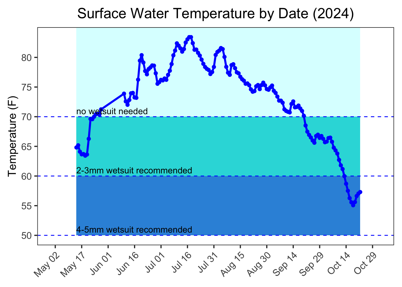
Another simple factor affecting a swimmer’s decision to enter urban waters is water temperature. Good news! For all of June, July, and August the surface water temperature was above 70 degrees Fahrenheit. For swimming in May or September, a 2-3mm wetsuit is recommended. In October, a 4-5mm wetsuit is recommended.

Code

ggplot(water2024_summary, aes(x = date, y = avg_temp)) +
  geom_rect(aes(xmin = min(date), xmax = max(date),
                ymin = 70, ymax = Inf),
            fill = "cadetblue1", alpha = 0.01) +
  geom_rect(aes(xmin = min(date), xmax = max(date),
                ymin = 60, ymax = 70),
            fill = "#17c3b2", alpha = 0.01) +
  geom_rect(aes(xmin = min(date), xmax = max(date),
                ymin = 50, ymax = 60),
            fill = "#1f77b4", alpha = 0.01) +
  geom_line(color = "blue", size = 1.2) +  # Thicker, clearer line
  geom_point(color = "blue", size = 1.8) +  # Larger points for clarity
    geom_hline(yintercept = 70, linetype = "dashed", color = "blue") +
  geom_hline(yintercept = 60, linetype = "dashed", color = "blue") +
  geom_hline(yintercept = 50, linetype = "dashed", color = "blue") +
    annotate("text", x = min(water2024_summary$date), y = 71,
           label = "no wetsuit needed", hjust = 0) +
  annotate("text", x = min(water2024_summary$date), y = 61,
           label = "2-3mm wetsuit recommended", hjust = 0) +
  annotate("text", x = min(water2024_summary$date), y = 51,
           label = "4-5mm wetsuit recommended", hjust = 0) +
  scale_y_continuous(breaks = seq(0, max(water2024_summary$avg_temp), by = 5)) +
  scale_x_date(
    limits = as.Date(c("2024-05-01", "2024-11-01")),
    date_labels = "%b %d", 
    date_breaks = "15 day"
  ) +
  labs(title = "Surface Water Temperature by Date (2024)",
       x = NULL,
       y = "Temperature (F)") +
  theme_bw(base_size = 15) +  # Larger base size for readability
  theme(
    plot.title = element_text(size = 18, hjust = 0.5),  # Title style
    axis.title = element_text(size = 14),  # Axis titles size
    axis.text = element_text(size = 12),  # Axis labels size
    axis.text.x = element_text(angle = 45, hjust = 1),  # Rotate X-axis labels for clarity
    panel.grid.major = element_blank(),  # Remove major grid lines
    panel.grid.minor = element_blank(),  # Remove minor grid lines
    plot.margin = margin(10, 10, 10, 10)  # Adjust margins for better spacing
  )

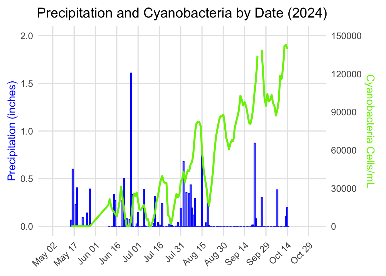
3.4 Is rainfall correlated with water quality?

Rainfall does not appear to be correlated with cyanobacteria levels. Other factors (e.g., nutrients, temperature) might play a more substantial role in driving variations in cyanobacteria, and rainfall may have a stronger correlation with fecal bacteria from sewage runoff (not included in this analysis).

Code

library(dplyr)
library(ggplot2)
library(tidyr)
library(lubridate)
library(scales)

weather2024<-read.csv('./data/weather2024daily.csv')
weather2024<-weather2024 |> 
  select(datetime,temp,precip)
weather2024$date<-as.Date(weather2024$datetime, format = "%Y-%m-%d")

weather_and_water_2024<-merge(water2024_summary, weather2024, by = 'date')

# PLOT
ggplot(weather_and_water_2024, aes(x = date)) +
  geom_col(aes(y = precip, color = "Precipitation"), fill = "blue", alpha = 0.5, width = 0.8) +
  geom_line(aes(y = avg_est_cyano / 75000, color = "Cyanobacteria Cells/mL"), size = 1.2) +
  scale_y_continuous(
    name = "Precipitation (inches)", 
    limits = c(0, 2), 
    breaks = seq(0, 2, 0.5),
    sec.axis = sec_axis(~.*75000, name = "Cyanobacteria Cells/mL", breaks = seq(0, 150000, 30000))
  ) +
  scale_x_date(
    limits = as.Date(c("2024-05-01", "2024-11-01")),
    date_labels = "%b %d", 
    date_breaks = "15 day"
  ) +
  scale_color_manual(values = c("Precipitation" = "blue", "Cyanobacteria Cells/mL" = "chartreuse2")) +
  labs(
    title = "Precipitation and Cyanobacteria by Date (2024)",
    x = NULL,
    color = "Variable"
  ) +
  theme_minimal(base_size = 15) +
  theme(
    plot.title = element_text(size = 18, hjust = 0.5),  # Title styling
    axis.title = element_text(size = 14),  # Axis labels styling
    axis.text = element_text(size = 12),  # Axis ticks styling
    axis.text.x = element_text(angle = 45, hjust = 1),  # Rotate X-axis labels for better readability
    axis.title.y.left = element_text(color = "blue", size = 14),  # Precipitation axis label color
    axis.title.y.right = element_text(color = "chartreuse2", size = 14),  # Cyanobacteria axis label color
    legend.position = "none",  # Remove legend for simplicity
    panel.grid.major = element_line(color = "gray90"),  # Slight grid lines for better visibility
    panel.grid.minor = element_blank(),  # No minor grid lines
    plot.margin = margin(10, 15, 10, 10)  # Adjust plot margins for clarity
  )

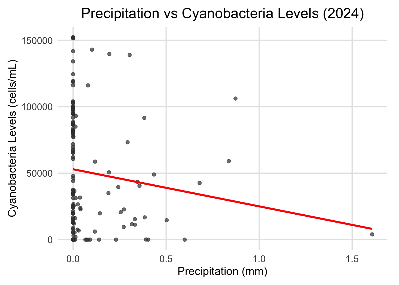
The Spearman correlation score for rainfall and cyanobacteria levels is -0.2879425, suggesting a weak negative correlation. This is the opposite of what we expected and should be investigated further, perhaps on a larger or more fine grained data set.

Code

ggplot(weather_and_water_2024, aes(x = precip, y = avg_est_cyano)) +
  geom_point(size = 1.8, alpha = 0.7, color = "#3b3b3b") +
  geom_smooth(method = "lm", se = FALSE, color = "red", size = 1.2) +
  labs(
    title = "Precipitation vs Cyanobacteria Levels (2024)", 
    x = "Precipitation (mm)", 
    y = "Cyanobacteria Levels (cells/mL)"
  ) +
  theme_minimal(base_size = 15) +  # Use minimal theme for a clean look
  theme(
    plot.title = element_text(size = 18, hjust = 0.5),  # Bold and centered title
    axis.title = element_text(size = 14),  # Axis titles size
    axis.text = element_text(size = 12),  # Axis tick labels size
    panel.grid.major = element_line(color = "gray90"),  # Light grid lines for readability
    panel.grid.minor = element_blank(),  # Remove minor grid lines for cleanliness
    plot.margin = margin(10, 15, 10, 10)  # Adjust margins for clarity
  )